This software is distributed under the GNU General Public Licence, version 2. For alternative licensing arrangements, contact the author, Matthew Belmonte.

If you base a publication on this software, please cite either the ACM newsletter publication mentioned in the source files, or (preferably), the first peer-reviewed article in which it was applied (follow the link).

The code described here was developed with a specific application in mind. However, many of the programs are more generally applicable. Here is a list of these general-purpose programs that you may find useful:

TRANSFORMATIONS
cntcat - concatenate .CNT files
lderiv - compute a linear derivation from a .CNT file
range - replace points in a .AVG file by local range measures
extreme - replace points in a .AVG file by local extrema
detrend - remove linear voltage trends from a .AVG file (a high-pass filter)
smooth - smooth a .AVG file (a low-pass filter)
rectify - replace points in a .AVG file by their absolute values
power - compute the power spectrum of a .AVG file in a moving window
addavg - compute the pointwise sum of two .AVG files
scale - scale a .AVG file
subepoch - extract a sub-interval from a .AVG file
ztrans - transform a .AVG file into z-scores, with variance and mean from another .AVG file

STATISTICS
chisquare - compute a Chi-square test on the .AVG output from ztrans
permtest - a permutation test applied to a group of .AVG files
ttest - apply Student's t test to a .AVG file
mannwhitney - the Mann-Whitney test applied pointwise to two sets of .AVG files
signtest - the sign test applied pointwise to a group of .AVG files
friedman - Friedman's rank test applied pointwise to a set of .AVG files

DUMPS
dumpavg - create an ASCII dump of a .AVG file
dumpevtb - create an ASCII dump of the event table of a .CNT file
plotavg - translate a .AVG file into PostScript code for printing

Only the "power" program requires the Numerical Recipes library to compile; the others depend only on public-domain libraries.

This paper focusses on the specific application for which Gnuroscan was developed, the analysis of steady-state evoked potentials. If you just want the software and aren't interested in steady-state evoked potentials, you may want to go directly to the download page.

DOWNLOAD REPRINT (requires password)

ABSTRACT: A suite of computer programs tailored to the analysis of steady-state evoked potential data in attentional shifting experiments is described. Stimuli are sequenced pseudorandomly while maintaining constraints on overlapping of response windows. Averages of phase-locked and non-phase-locked steady-state amplitudes are computed in variable-length epochs and corrected for the effect of sampling noise. Various algebraic and combinational transformations of averaged data are implemented. Several parametric and nonparametric statistical tests are implemented, and the results of these procedures are visualised. An application of this software has revealed modulation of a steady-state visual evoked potential by spatial attention. The software has been designed with portability in mind, and many of the programs are applicable to more general problems in evoked potentials.

Descriptors: EEG, Steady-State Evoked Potential, Software

INTRODUCTION

A steady-state evoked potential (SSEP) is a continuously oscillatory potential generated by the brain in response to a periodic driving stimulus. Particularly good resonances are observed for the visual SSEP when stimuli are flashed at about 10s^-1 [Fedotchev & al. 1990] and for the auditory SSEP when clicks occur at about 40s^-1 [Galambos & al. 1981]. Perturbations of the SSEP from its background amplitude and phase indicate changes in brain state. The SSEP has been used to index the salience of stimuli in studies of auditory perception [Rohrbaugh & al. 1989; Galambos & Makeig 1992] and visual perception [Allen & al. 1986; Chen & al. 1990; Bach & Meigen 1992; Snowden & al. 1995], and as an indicator of the degree of involvement of cortex in cognitive processing tasks [Silberstein & al. 1990, 1995]. The rapid, regularly timed, and ongoing nature of SSEP resonances makes them useful in such applications. The temporal resolution of SSEP measurements depends upon the frequency of the driving input and is bounded by the switching times of the neural networks involved in generating the SSEP and by the modulation transfer functions of the overlying tissues and sensors.

In tasks that require some behavioural response, the stimuli that drive the SSEP may or may not be identical with the stimuli to be evaluated for response. A target stimulus such as a tone or a picture can perturb an SSEP driven by an ongoing sequence of background stimuli such as clicks or flashes. Alternatively, the properties of the background stimuli themselves can be modulated in order to provide a target stimulus. For example, in an experiment involving a visual SSEP, a colour change in one of a series of periodic flashes can indicate a target. Stimuli consist of a series of instances of the background stimulus punctuated by instances of the target stimulus. The evoked responses consist not only of the response to the single, target stimulus, but also of perturbations in the overlapping responses to the surrounding background stimuli.

A logical extension of the application of SSEPs as measures of perception within sensory channels is their use in experiments involving the shifting or reallocation of attention between sensory channels. These two different channels might be spatial locations, spatial frequencies, colours, pitches, or even different sensory modalities. In our test experiment, the two sensory channels were defined by spatial location. The behavioural task essentially was two visual oddball paradigms running side by side in two different spatial locations; a target stimulus in one location cued not only an overt, behavioural response but also a shift of attention to the other, concurrently running oddball series. The next target in this newly attended series then cued a shift back to the original location, and so on. The initial, immediately practical goal of this project was to design a software system capable of processing SSEP responses in this paradigm.

BACKGROUND

Most conventional software for the processing of evoked potentials is tailored to a single-stimulus format, in which stimuli are delivered in isolated instances and the evoked response is a single, self-contained waveform rather than a perturbation of an ongoing waveform. Also, since target stimuli generally occur in separate experimental trials from each other, the length of the averaging epoch in teach trial is unbounded by neighbouring targets, and therefore an epoch of constant length is assumed. Methods of data reduction and statistical evaluation usually are not handled by such software systems, and instead must be specified by the experimenter explicitly. Finally, there is some difficulty in combining modules in an off-the-shelf manner in order to automate data processing.

Newer software systems have made some progress against many of the aforementioned shortcomings. A commercial system in widespread use in evoked potential laboratories, SCAN (NeuroScan, El Paso, Texas) was used as the basis for this system. SCAN includes a basic toolkit for the analysis of evoked potentials, and a batch scripting language that allows automation of many of the processing steps by modular combination of various subprograms from this toolkit. Nevertheless, many users of SCAN still employ custom, in-house software for the less standard and more arcane aspects of their data processing. In particular, the difficulties of the single-stimulus format, the constant-length averaging epoch, and the manual nature of data reduction and statistical evaluation remain to be addressed.

DESIGN CONSIDERATIONS

The goal of the project reported here was to construct an evoked potential processing system tailored to steady-state applications but also applicable to other problems in signal processing. Realistic assumptions of the computing power commonly available in the 1990s were made: the system tends to trade computational tractability for exactness of results. A benefit of this trade-off is that few assumptions about the statistical character of the data need be made; for example, the nonparametric statistical routines produce valid results even when the data are asymmetrically distributed. There is an `off-the-shelf' modularity to the system: single operations such as linear transformation, scoring, averaging, statistical analyses, and visualisation are implemented as separate programs. This ease of combining the several utilities in the Gnuroscan toolkit leaves the investigator free to deal with scientific questions rather than becoming caught up in the specifics of algorithmic designs and software implementations.

Because I was starting from the basis provided by the SCAN software, the analysis software described herein, `Gnuroscan', has been implemented to conform to SCAN's data file formats, but these are easily translated into other representations. Portability, modularity, and extensibility of the software were major goals. The entire system has been implemented in ANSI standard C language, and all graphical output has been implemented using the standard display language PostScript. Details on the data format, the algorithms, and the implementation details are available in order to allow extension and customisation of the software by other investigators. The software, including source code, is available from the author.

SYSTEM DESCRIPTION

Sequencing and presentation of stimuli. Before data can be gathered in such an attentional-shift experiment, the stimuli to be delivered in each sensory channel (in the case of our test experiment, in each spatial location) must be sequenced. The position in which a stimulus occurs within a sequence of stimuli determines the bounds of its response window, that is, the time interval within which a behavioural response to that stimulus may occur. A shortcoming of previous experiments involving rapidly repeated shifts of attention back and forth between two different sensory channels [Akshoomoff & Courchesne 1992; Courchesne & al. 1994a, 1994b] has been the difficulty in mapping responses unambiguously to particular stimuli, due to overlaps of response windows. Typically, a response is scored as a hit or as a false alarm depending on whether it occurs within the response window following the delivery of a target stimulus. The interval between the onset of the target and the opening of this window, [Delta]t_open, typically some 200ms, is assumed to be the minimum behavioural reaction time that would be physiologically possible. The interval between the onset of the target and the closing of this window, [Delta]t_close, 1400ms in the experiments cited, is assumed to be the maximum possible latency of a response. However, an ambiguity ensues if the response windows for two successive targets overlap; it is not immediately clear which target a particular response should be associated with. Such conflicts can be resolved using heuristics, for instance by associating each response with the most recent target within whose window the response lies.

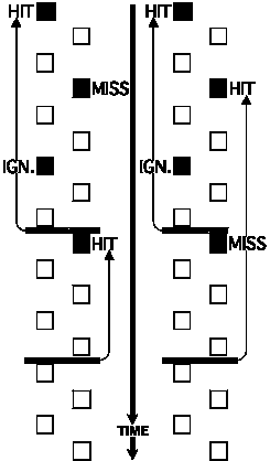An ambiguity still ensues, however, in the case in which the response window for a missed target overlaps the response window for a correctly detected target in the same sensory channel. In such a situation, the response cannot be mapped unequivocally to either of the targets. In the current implementation of the Gnuroscan system, targets alternate between only two sensory channels. In order to refer to a concrete example, this discussion will use the case of a spatial attention experiment in which the two channels correspond to the two sides of space. So, in this example, targets alternate between the left side and the right side. Therefore, successive targets on the same side are separated by the sum of two successive intertarget intervals. Call these intervals t_i and t_i+1, respectively. Let T be the time of occurrence of the first target of interest. Then the time of occurrence of the next target on the same side is T+t_i+t_i+1. In order for the response windows not to overlap, the end of the first window, T+[Delta]t_close, must not be greater than the beginning of the next window, T+t_i+t_i+1+[Delta]t_open. This constraint can be accomplished by generating the sequence of intertarget intervals using a Markov chain to derive a pseudo-uniform distribution (subject to whatever discretisation is required by the experimental paradigm or by the stimulus delivery hardware) of intertarget intervals t over some interval [0, t_max] conditioned to t_i+t_i+1 >= [Delta]t_close-[Delta]t_open. This method is applied off-line, by the sequence program, to compute a stimulus sequence which is fed to a separate stimulus-delivery program.

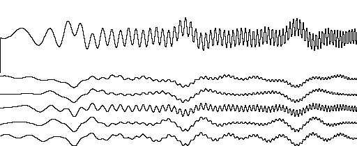Transformation of raw data. Once the raw data have been collected, the computation begins in earnest. In many analyses, the first step is to convert the data from the physical recording channels to some linear combination of the original channels. Examples of this are re-referencing, transformation between bipolar and common-reference recordings, and Hjorth's [1975] approximation to the discrete Laplacian transformation. The cntcat program catenates separate files of continuous EEG data, and the lderiv program computes an arbitrary linear combination of channels from a raw data file.

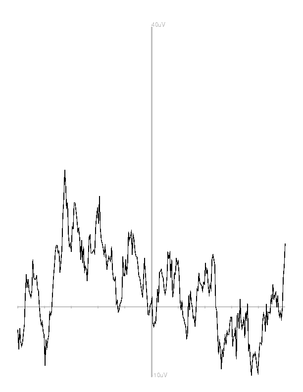Rejection and scoring. The score program assumes that the horizontal and vertical electrooculograms are available as part of the recorded electrophysiological data. (These may be virtual channels, derived as a linear combination of recording channels.) It computes the median of the horizontal electrooculuogram in a moving window. Because some phasic activity from the steady-state potential will leak into the eye channels, it's important that the length of this window be an integral number of interstimulus intervals. This prevents the biasing of the median by such phasic activity and thus yields a less variable signal of eye position. When the range of this signal within a local neighbourhood exceeds a threshold, a horizontal saccade is detected. In the test experiment, useful values for the length of the median filter window, the size of the local neighbourhood, and the rejection threshold were, respectively, 336ms (three complete interstimulus intervals), 75ms (a liberal figure for the duration of a saccade), and 25uV.

A similar method is applied to the vertical electrooculogram in order to detect blinks. Because the amplitude of the blink signal recorded near the orbit is strictly greater than the amplitude of the SSEP, the length of the median filter window need not be an integral number of interstimulus intervals in this case. In the test experiment, useful values for the length of the median filter window, the size of the local neighbourhood, and the rejection threshold were, respectively, 75ms, 300ms, and 100uV. Gnuroscan includes an option for calculating the voltage thresholds automatically from calibrations marked in the event record.

All this repetitive computation of medians in moving windows is optimised using a combination of queues and binary search trees. A queue keeps track of the order of samples within a window, and a binary search tree enables the implementation of insertion, deletion, and computation of the median in O(log w) time, where w is the length of the window. Thus, for a record comprising n digital samples, the entire record can be scanned for ocular artefacts in O(n log w) time.

The scoring program also assumes that each stimulus and each response are marked by an event code inserted in the record. Due to the very high rate of data transfer in SSVEP experiments, with the spacing between event codes sometimes being as little as a few milliseconds, the software includes checks for omitted or mis-transcribed event codes. The commercial software used for data acquisition in our test case did indeed drop some codes, and mis-transcribed others. These errors probably were due to imperfect synchronisation of the read operation in the computer that was recording the data with a strobe signal from the computer that was supplying the event codes. Whatever the source of the errors, their presence demonstrates the importance of this check. Isolated corruptions of event codes almost always can be repaired by utilising redundancies in the data. In our spatial attention example, suppose the subject is responding to targets in alternate hemifields by moving a joystick between the two sides of space. In such a situation, it's impossible for two joystick movements in the same direction to occur without a joystick movement in the opposite direction between them. For instance, if the joystick makes a transition from the right side to the left side, it must first return from the left side to the right side before another transition from right to left can be recorded. So for each target, if a response occurs within the current response window, and this response hasn't already been associated with some prior target, the response is treated as a correct response to the current target even if its recorded laterality is incorrect. In such a case, the event code is rewritten with the appropriate laterality. In cases in which the response code is completely dropped, the response latency cannot be recovered, but the fact that a response did occur is still evident, because the omitted response will cause the juxtaposition of two responses that are on the same side as each other.

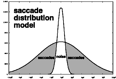A separate program, eyehand, extracts correlations of horizontal eye movements with manual responses. The distribution of amplitudes of maximal-length nondecreasing or nonincreasing intervals of the horizontal electrooculogram is modelled as the sum of two zero-mean Gaussians, one of them accounting for noise and microsaccades, and the other accounting for larger-amplitude saccades of the type that often occur in response to a cue to shift attention. The Levenberg-Marquardt algorithm [Press & al. 1992] is used to zero in on the parameters that define these Gaussians. The absolute value at which these two Gaussian curves cross is computed and used as a threshold. The saccade latency in response to a target is defined as the latency of the beginning of the first nondecreasing or nonincreasing interval whose range exceeds the threshold and whose direction is the same as the direction of the attentional shift cued by the target. Correlations and regression coefficients are then computed to describe the relationship between saccade latency and latency of manual responses.

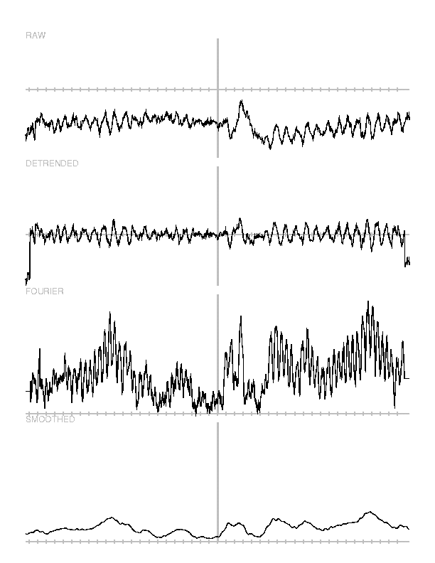Averaging. The average program is the heart of the Gnuroscan system. It computes averages both of instantaneous amplitude and of amplitude within certain frequency bands in a local neighbourhood. Instantaneous amplitude is calculated by the simple, time-domain averaging procedure that is widely used in studies of event-related potentials. Amplitude specific to certain frequency bands is computed by subjecting each single-trial, time-domain signal to a Fast Fourier Transform (FFT) [Press & al. 1992], and then calculating the length of the vector formed by the Fourier sine and cosine coefficients at the frequency or frequencies of interest. The signal is prepared for the FFT by resampling an interval whose length is one complete interstimulus period so that the resulting number of samples within this interval is a power of two, and by detrending and convolution with a cosine-bell window to prevent spectral leakage. The vector length of the FFT coefficients is then the amplitude of the signal at the frequency of interest within a one-stimulus-cycle neighbourhood centred on the current time point. The FFT interval is stepped through the data in order to compute successive frequency-specific amplitudes centred on each time point within the epoch.

The detrending operation and the windowed amplitude calculation are also implemented as separate, self-contained programs (detrend and power), outside of the averaging program. These are used to transform the instantaneous amplitude averages, which were calculated previously, into moving-window amplitudes at the frequencies of interest. Why do it both ways? Why calculate both an average of the single-trial frequency-specific amplitudes and the frequency-specific amplitudes of a time-domain average? It turns out that the operations of averaging and of computing the frequency-specific amplitude are not commutative. That is, one obtains different results when the amplitude calculation occurs before the averaging than when the averaging occurs before the amplitude calculation. This is because the amplitude calculation, depending as it does on a two-dimensional distance relation, is a non-linear operation. Averaging over sufficiently many trials eliminates (most of) the variance due to noise and leaves only the variance due to signal. Noise, in this sense, consists both of instrument noise and of background EEG whose phase is not time-locked to stimulus presentation. Thus the amplitudes calculated from the time-domain averages reflect phase-locked activity at each frequency of interest, whereas the averages of the single-trial amplitudes reflect total activity, including activity that is not phase-locked. Both these measures are of interest.

In attempting to maximise signal-to-noise ratio from the data available, another difficulty arises. In order to squelch as much noise as possible, all available samples at any particular time point must be included in the averages. But since the length of time since the previous shift of attention and the length of time until the next shift of attention vary across different instances of targets, the epoch length is not constant. The average can still be computed, by alligning all epochs to the time of target delivery and using a separate divisor for each time point. But this creates a secondary problem. The signal-to-noise ratio varies as the square root of the number of samples in the average. Using this scheme, the number of samples decreases towards the ends of the maximal-length epoch. So the variance of the signal, and therefore the amplitude at any particular frequency, is biased upward toward the ends of the epoch. In pictorial terms, the amplitude function versus time is concave downward, with a minimum at the centre of the epoch. This bias can be corrected by using the baseline, that is, the half of the epoch before the time of target delivery, as a model of the bias. The local range of the signal over one complete stimulus cycle is fit to the function

with parameters p₀ and p₁ and number of observations n, using the Levenberg-Marquardt algorithm. In the expression above, the left-hand factor of each term determines the relative contribution of the corresponding right-hand factor. The two left-hand factors are complementary, having unit sum. They are sigmoid functions that implement a rather abrupt, yet continuous (and so differentiable) switch between dominance of the left-hand term at high n and dominance of the right-hand term at low n. When the value of n, the number of observations in the average, is high, it has little effect on the range of the signal. Conversely, when n is low, noise biases the amplitude upward with an inverse dependency on the square root of n. The fitted parameter p₀ is the critical value of n at which the inverse-square-root, noise-related amplitude level begins to dominate the constant, asymptotic amplitude level. The noise correction factor for some particular number of observations n_t is then

In addition to computing these averages for each combination of target channel, response accuracy, and length of time since the most recent shift, the averaging routine calculates the vector of standard deviations associated with each average, reports average response latency and its standard deviation for each sensory channel and for several separate ranges of inter-target intervals, and computes histograms of the amplitude of the horizontal electrooculogram versus time during attentional shifts.

Transformations of averaged files. Several programs are provided in order to implement algebraic and combinational operations on averaged data files. The most basic of these are addavg and scale. addavg takes a list of averaged files and produces an averaged file that is the pointwise sum of all these inputs. scale takes a scalar value and an averaged file and produces the averaged file that is the product of these two inputs. scale can be applied with a negative scalar and followed by addavg in order to implement substraction. scale can be applied with a reciprocal scalar and preceded by addavg in order to construct a grand average.

The subepoch program truncates an averaged data file at either end. This is useful in situations in which the epoch includes data points that are unused in the current analysis. The smooth program replaces each data point by the average of all the data points within a user-specifiable time window centred on the current data point. Smoothing is usefully applied to the output of the power program in order to damp ringing. A useful smoothing window in this situation is one fourth the length of the Fourier transform window. The rectify program replaces each data point with its absolute value. This is useful for examining signals such as difference waves, in which the important feature is the degree of deviation from zero. The range program replaces each data point with the local range of the signal within a user-specifiable time window centred on the current data point. This is a measure of local amplitude at frequencies whose periods are comparable to the length of the window.

Statistical analyses. In what follows, I use the ideas of data matrices and probability matrices. A data matrix is the structure quite familiar to all evoked potential researchers: it's what I was referring to above as an averaged data file. If the sampling epoch contains n data points, and c channels are being recorded, the result of averaging the electrophysiological responses to each target event is a cxn matrix of potentials. Thus the data matrix describes the actual perturbations of the electroencephalogram over time. These perturbations are superpositions of experimental effects and noise, and it isn't explicit from the data matrix alone which is which. In order to represent the levels of statistical significance of perturbations in the electroencephalogram, Gnuroscan uses a probability matrix. The probability matrix is another cxn matrix which maps strightforwardly onto the data matrix. Instead of potentials, though, the entries in the probability matrix are levels of statistical significance. These probabilities may be calculated by any of Gnuroscan's several statistical programs. Probability matrices are stored in the same format as data matrices and therefore may be viewed and manipulated with any of the tools that view and manipulate data matrices. In particular, applications needing a Bonferroni correction for multiple comparisons may implement this by applying the scale program to the probability matrix.

The ttest program implements a pointwise Student's t test on a set of data matrices, and produces a probability matrix. The inputs are treated as difference waves, and tested for significant deviation from zero. This simple test is useful when examining a single hypothesis or comparison.

The chisquare program operates on z-transformed data matrices. It uses a ² test to determine whether the set of z-scores differs significantly from samples that might be expected from the standard normal distribution. A significant probability value indicates that the stimulus does perturb the EEG, but not necessarily that it perturbs the EEG in a consistent manner: a stimulus that causes an amplitude increase in half the subjects and an amplitude decrease in the other half, for example, would still produce a significant ² probability even though the mean post-stimulus amplitude would still be within the pre-stimulus baseline range. This is a useful test when one is comparing only two treatments or conditions. As a preprocessing step to this procedure, the ztrans program transforms a data matrix to z-scores with respect to the mean and variance of a baseline data matrix. Depending on the design of the experiment, the baseline may be a subinterval of the epoch under consideration, or it may be a separate average. A baseline interval may be extracted from a longer epoch by means of the subepoch program.

The ² test is fine for a first cut, but it has two major shortcomings: by itself it fails to differentiate between differences in variance (inconsistent perturbations) and differences in mean (consistent perturbations), and it assumes that the distribution of individual amplitude perturbations is normal. A more versatile test, given the speed of today's electronic computers, is a permutation test. Often one desires to check whether the event-related potentials or perturbations of one experimental group differ from another, or from a control group. The usual way of accomplishing this is Fisher's F-test. Nonparametric methods, however, are more accurate and often more powerful than such resorts, because they have no need for an assumption of normality. The permutation test is the most straightforward of these. It compares the mean of the experimental group to the means of all possible samples drawn from the pooled groups that are of the same size as the experimental group. The ratio of the number of means less eccentric than the experimental mean to the total number of means is the probability of the null hypothesis. Gnuroscan implements a pointwise, exhaustive permutation test (the permtest program), using Chase's [1970] algorithm for generating all possible combinations of a given size. For cases in which the number of possible combinations is prohibitively large, a Monte Carlo version of this test also is available. (In the default configuration this critical value is set to 10⁵ combinations, but it can be tuned according to the speed of floating-point computations on the implementation system.)

Another useful nonparametric test is the sign test, implemented by the signtest program. This procedure applies the binomial probabilities to the sign of the signal. It's most usefully applied to difference waves between two experimental conditions, where, under the null hypothesis, positive and negative differences are equally likely at any given point in the epoch. A useful preprocessing step for this pointwise sign test is the transformation of the difference wave with the extreme program, which filters the input such that each point in the epoch is replaced by the point within a local window whose absolute value is largest. When the width of the local window is the period of the SSEP, this transformation has the effect of lining up the peak amplitudes across all the subjects, thus increasing the power of this pointwise test. Assuming that noise is symmetrically distributed with zero mean--a fairly safe assumption in a difference wave--the probability of positive sign remains one half even after this transformation, and therefore the sign test still applies.

The mannwhitney program, like the permtest program, compares two groups of data matrices. A pointwise Mann-Whitney U test is used. The current implementation does not produce a probability matrix automatically, but such a matrix may be constructed from the matrix of U values that is output, using a standard statistical table. Applications of this program include comparison of a control group and an experimental group, and also comparisons of two treatment conditions within a single group of subjects.

The friedman program applies Friedman's test for a randomised block design to a group of subjects each of whom receives each of several experimental treatments. (Thus the individual subjects are the `blocks'.) This is useful in cases in which there are several levels of the experimental condition--for example, stimulus onset ansynchrony in a Posner-style attention task--and each of those conditions is applied to each subject. The mannwhitney program may be used as a pairwise post hoc test in cases in which Friedman's test indicates significant variation.

Visualisation. Gnuroscan provides three visualisation routines, all of which share characteristics. Each of these plotting programs produces a PostScript program from a group of data matrices. The image coded by this output program respresents variations in the signal and also the significance levels of those variations.

plotavg uses Efron's [1982] bootstrap procedure to construct a distribution for each channel from points in a baseline immediately prior to the zero time point of the epoch. The bootstrap estimates the shape of the distribution by repeatedly calculating means of subsets of the data points drawn with replacement. This resampling procedure is computationally more intensive than parametric procedures, but, assuming sufficient length of the baseline interval from which the distribution is constructed, it yields a more accurate representation of the actual distribution. The length of the baseline may be tuned according to the needs of the particular application. Significant (p<0.05, two-tailed) deviations from this bootstrapped baseline distribution are plotted in shades of dark grey whose intensities correspond to the significance level. Non-significant deviations are plotted in light grey.

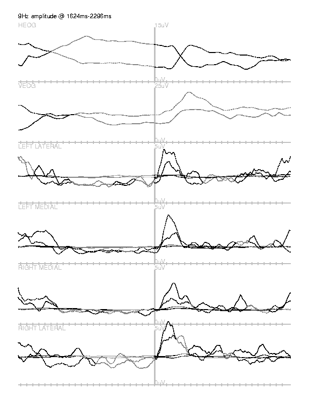fplotavg also uses a nonparametric, combinational statistical test, but its measure is the integral of a difference wave rather than the magnitude of the current sample. Its parameters are pairs of data matrices. For each pair, the difference wave is computed. The measure of difference is the integral between zero-crossings of this difference wave, in each channel. In order to estimate the magnitudes of such integrals due to random fluctuations, the prestimulus baselines are slid along each other in a Monte Carlo manner and the magnitudes of the integrals between zero-crossings of the resulting difference wave are computed in order to establish an empirical distribution. Poststimulus integrals are then ranked within this distribution in order to ascertain their significance.

zplotavg plots a single data matrix. Like the other plotting programs, it codes the significance level of each point as a grey level in the image. Unlike these other programs, though, it reads the significance levels from an accompanying probability matrix rather than computing them itself. Thus zplotavg is quite useful in combination with output from the separate statistical programs mentioned above.

STATUS REPORT

Taken together, these utilities form a flexible toolkit for the manipulation of averaged electroencephalographic data. The scoring and averaging routines are specific to the SSEP paradigm, but the other routines--transformations, statistical tests, and visualisation programs--are applicable to any problem in biological signal analysis.

The Gnuroscan system has been applied in a study of visual spatial attention [Belmonte 1998]. This study found significant perturbations of both phase-locked and non-phase-locked amplitude in various time intervals following the presentation of a stimulus that cued a voluntary shift of visual spatial attention. We hypothesise that these perturbations reflect the neural processes underlying orienting to a stimulus, reorienting to a new location, and distributing attention in anticipation of a subsequent shift. Although the effects of static allocation of visual spatial attention have been investigated using event-related potentials, this is the first study to apply detailed ERP measures to rapidly repetitive shifts in visual spatial attention.

LESSONS LEARNT

Several innovations implemented in the Gnuroscan system have been valuable in analysis of steady-state evoked potentials and have avoided the pitfalls created by the rapid stimulus delivery which is essential in steady-state paradigms. Probabilistic constraints on pseudorandom stimulus sequencing enable unambiguous mapping of behavioural responses to particular target stimuli, even when the stimulus presentation rate is quite high. Redundancy in coding of behavioural responses allows reconstruction of behavioural data that are lost during rapid transfers. The use of variable-length epochs in the averaging routine makes maximal use of the steady-state response recorded between each pair of target stimuli, and the inhomogeneity of sampling noise introduced by this feature can be compensated for.

In addition, several of Gnuroscan's features have impact beyond the scope of SSEPs. Fast digital filters automate the detection of saccades and blinks that may be produced in response to rapid stimuli. Separate analyses of phase-locked and non-phase-locked responses yield complementary information about the neurophysiological processes associated with stimulus perception. Nonparametric statistical tests, some of which can involve very substantial amounts of computation, can give more exact and valid information on the significance of the effects observed.

FUTURE PLANS

The focus in this work has been on development of the underlying algorithms. Gnuroscan's user interface, therefore, is minimal, and is entirely text-based. A priority in future development work will be to add a versatile, graphical front end as a user interface to all of Gnuroscan's subprograms. In addition, many statistical routines remain to be implemented; development of the existing set of statistical programs was driven by immediate need for them in a research application. The possibility exists for the development of an interface to a commercial statistical package. Finally, in order to see the widest possible application, future versions of Gnuroscan will have to include translators that convert between the SCAN format and other major formats for the storage of digital electroencephalographic data.

ACKNOWLEDGEMENTS

I thank Eric Courchesne of the Autism and Brain Development Research Laboratory for providing facilities and financial support for part of this work, and, more importantly, for his friendship which spanned most of my time in San Diego. I also thank Brian Egaas of Science Applications International Corporation for teaching me the finer points of signal processing, Bruce Fischer of the MIT Mathematics Department for suggesting conditioned distributions as a way to implement constraints on pseudorandom inter-target intervals, Anthony Gamst of the UCSD Mathematics Department for suggesting a more powerful, computational alternative to parametric statistics for the analysis of moving-window amplitudes, and Robert Ringrose of the MIT Artificial Intelligence Laboratory for providing computing facilities for the latter part of this work.

BIBLIOGRAPHY

Natacha Akshoomoff, Eric Courchesne, `A New Role for the Cerebellum in Cognitive Operations', Behavioral Neuroscience 106:5:731-738 (1992).

D Allen, AM Norcia, CW Tyler, `Comparative Study of Electrophysiological and Psychophysical Measurement of the Contrast Sensitivity Function in Humans', American Journal of Optometry and Physiological Optics 63:6:442-449 (1986).

M Bach, T Meigen, `Electrophysiological Correlates of Texture Segregation in the Human Visual Evoked Potential', Vision Research 32:3:417-424 (1992).

Matthew Belmonte, `Shifts of Visual Spatial Attention Modulate a Steady-State Visual Evoked Potential', Cognitive Brain Research 6:4:295-307 (1998).

Phillip J Chase, `Algorithm 382: Combinations of M out of N Objects [G6]', Communications of the Association for Computing Machinery 13:6:368 (1970).

SA Chen, LZ Wu, DZ Wu, `Objective Measurement of Contrast Sensitivity Using the Steady-State Visual Evoked Potential', Documenta Ophthalmologica 75:2:145-153 (1990).

Eric Courchesne, Jeanne Townsend, Natacha Akshoomoff, Rachel Yeung-Courchesne, Alan Lincoln, Gary Press, James Murakami, Hector James, Osamu Saitoh, Brian Egaas, Richard Haas, Laura Schreibman, `A New Finding: Impairment in Shifting Attention in Autistic and Cerebellar Patients'. In: SH Broman & J Grafman (eds.), Atypical Cognitive Deficits in Developmental Disorders: Implications for Brain Function (Hillsdale, New Jersey: Lawrence Erlbaum, 1994a), 101-137.

Eric Courchesne, Jeanne Townsend, Natacha Akshoomoff, Osamu Saitoh, Rachel Yeung-Courchesne, Alan Lincoln, Hector James, Richard Haas; Laura Schreibman, Lily Lau, `Impairment in Shifting Attention in Autistic and Cerebellar Patients', Behavioral Neuroscience 108:5:848-865 (1994b).

Bradley Efron, The Jackknife, the Bootstrap and Other Resampling Plans. Philadelphia: Society for Industrial and Applied Mathematics, 1982.

Alexander I Fedotchev, Alexander T Bondar, Vladimir F Konovalov, `Stability of resonance EEG reactions to flickering light in humans', International Journal of Psychophysiology 9:2:189-193 (1990).

Robert Galambos, Scott Makeig, `Physiological Studies of Central Masking in Man. I: The Effects of Noise on the 40-Hz Steady-State Response', Journal of the Acoustical Society of America 92:5:2683-2690 (1992).

Robert Galambos, Scott Makeig, PJ Talmachoff, `A 40-Hz Auditory Potential Recorded from the Human Scalp', Proceedings of the National Academy of Sciences 78:4:2643-2647 (1981).

Bo Hjorth, `An On-Line Transformation of EEG Scalp Potentials into Orthogonal Source Derivations', Electroencephalography and Clinical Neurophysiology 39:5:526-530 (1975).

William H Press, Saul A Teukolsky, William T Vetterling, Brian P Flannery, Numerical Recipes in C: the art of scientific computing 2/e. New York: Cambridge University Press, 1992.

JW Rohrbaugh, JL Varner, SR Paige, MJ Eckardt, RJ Ellingson, `Event-Related Perturbations in an Electrophysiological Measure of Auditory Function: a Measure of Sensitivity during Orienting?', Biological Psychology 29:3:247-271 (1989).

Richard B Silberstein, Mark A Schier, Andrew Pipingas, Joseph Ciorciari, Stephen R Wood, David G Simpson, `Steady-State Visually Evoked Potential Topography Associated with a Visual Vigilance Task', Brain Topography 3:2:337-347 (1990).

Richard B Silberstein, Joseph Ciorciari, Andrew Pipingas, `Steady-state visually evoked potential topography during the Wisconsin card sorting test', Electroencephalography and Clinical Neurophysiology 96:1:24-35 (1995).

RJ Snowden, D Ullrich, M Bach, `Isolation and Characteristics of a Steady-State Visually-Evoked Potential in Humans Related to the Motion of a Stimulus', Vision Research 35:10:1365-1373 (1995).